
Although we have not formally discussed the issue of statistical power, the general idea has come up many times. In the SPSS examples we've worked through, we sometimes have observed what look like small relationships or differences, but which have turned out to be statistically significant due to a large sample size. In other words, large sample sizes give you statistical power.
In research, our aim is to detect a statistically significant relationship (i.e., reject the null hypothesis) when the results warrant such. Therefore, my personal definition of statistical power boils down to just four words:
Detecting something that's there.
I also like to think in terms of a biologist attempting to detect some specimen with a microscope. Two things can aid in such detection: A stronger microscope (e.g., more powerful lenses, advanced technology) or a visually more apparent (e.g., clearer, darker, brighter) specimen.
The analogy to our research is that greater statistical power is like increasing the strength of the microscope. According to King, Rosopa, & Minium (2011), "The selection of sample size is the simplest method of increasing power" (p. 222). There are, however, additional ways to increase statistical power besides increasing sample size.
Further, a stronger relationship in the data (e.g., a .70 correlation as opposed to .30, or a 10-point difference between two means as opposed to a 2.5-point difference) is like a more visually apparent specimen. Strength of the results is also somewhat under the control of the researchers, who can take steps such as using the most reliable and valid measures possible, avoiding range restriction when designing a correlational study, etc.
The calculation of statistical power can be informed by the following example. Suppose an investigator is trying to detect the presence or absence of something. For example, during the Olympics all athletes (or at least the medalists) will be tested for the presence or absence of banned substances in their bodies. Any given athlete either will or will not actually have a banned substance in his or her body (“true state”). The Olympic official, relying upon the test results, will render a judgment as to whether the athlete has or has not tested positive for banned substances (the decision). All the possible combinations of true states and human decisions can be modeled as followed (format based loosely on Hays, W.L., 1981, Statistics, 3rd ed.):
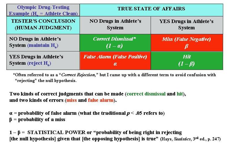
[Notes: The term “alpha” for a scale’s reliability is something completely separate and different from the present context. Also, the terms “Type I” and “Type II” error are sometimes used to refer, respectively, to false alarms and misses; I personally boycott the terms “Type I” and “Type II” because I feel they are very arbitrary, whereas you can reason out what a false alarm or miss is.]
For the kind of research you’ll probably be doing...
“The power of a test is the ability of a statistical test with a specified number of cases to detect a significant relationship.”
(Original source document for above quote no longer available online.)
Thus, you’re concerned with the presence or absence of a significant relationship between your variables, rather than the presence or absence of drugs in an athlete’s body.
(Another term that means the same as statistical power is "sensitivity.")
This document makes two important points:
*There seems to be a consensus that the desired level of statistical power is at least .80 (i.e., if a signal is truly present, we should have at least an 80% probability of detecting it; note that random sampling error can introduce "noise" into our observations).
*Before you initiate a study, you can calculate the necessary sample size for a given level of power, or, if you're doing secondary analyses with an existing dataset, for example, you can calculate the power for the existing sample size. As the linked document notes, such calculations require you to input a number of study properties.
One that you'll be asked for is the expected "effect size" (i.e., strength or magnitude of relationship). Here's where Cohen's classification of small, medium, and large correlations comes in handy. I suggest being cautious and assuming you'll discover only a small relationship in your upcoming study. For comparing two means, remember that the t-test is used only for determining statistical significance (i.e., seeing where your result falls on the t distribution). Thus, for a two-group comparison of means, you have to use something called "Cohen's d" for seeing what a small, medium, and large difference between means (or effect size) would be. Cohen's (1988) book Statistical Power Analysis for the Behavioral Sciences (2nd Ed.) conveys his thinking on what constitute small, medium, and large differences between groups...
Note that there's always a trade-off between reducing one type of error and increasing the other type. As King et al. (2011) explain, "In general, reducing the risk of Type I error [false alarm] increases the risk of committing a Type II error [miss] and thus reduces the power of the test" (p. 223). Consider the implications of using a .05 or .01 significance cut-off. The .01 level makes it harder to declare a result "significant," thus guarding against a potential false alarm. However, making it harder to claim a significant result does what to the likelihood of the other type of error, a miss? What is the trade-off when we use a .05 significance level?
Power-related calculations can be done using online calculators (e.g., here, here, and here). There are power calculators specific to each type of statistical technique (e.g., power for correlational analysis, power for t-tests).
More power to you!
This document makes two important points:
*There seems to be a consensus that the desired level of statistical power is at least .80 (i.e., if a signal is truly present, we should have at least an 80% probability of detecting it; note that random sampling error can introduce "noise" into our observations).
*Before you initiate a study, you can calculate the necessary sample size for a given level of power, or, if you're doing secondary analyses with an existing dataset, for example, you can calculate the power for the existing sample size. As the linked document notes, such calculations require you to input a number of study properties.
One that you'll be asked for is the expected "effect size" (i.e., strength or magnitude of relationship). Here's where Cohen's classification of small, medium, and large correlations comes in handy. I suggest being cautious and assuming you'll discover only a small relationship in your upcoming study. For comparing two means, remember that the t-test is used only for determining statistical significance (i.e., seeing where your result falls on the t distribution). Thus, for a two-group comparison of means, you have to use something called "Cohen's d" for seeing what a small, medium, and large difference between means (or effect size) would be. Cohen's (1988) book Statistical Power Analysis for the Behavioral Sciences (2nd Ed.) conveys his thinking on what constitute small, medium, and large differences between groups...
Small/Cohen's d = .20
"...approximately the size of the difference in mean height between 15- and 16-year-old girls (i.e., .5 in. where the [sigma symbol for SD] is about 2.1)..." (Cohen p. 26).
|
Medium/Cohen's d = .50
"A medium effect size is conceived as one large enough to be visible to the naked eye. That is, in the course of normal experience, one would become aware of an average difference in IQ between clerical and semiskilled workers or between members of professional and managerial occupational groups (Super, 1949, p. 98)" (Cohen, p. 26). |
Large/Cohen's d = .80
"Such a separation, for example, is represented by the mean IQ difference estimated between holders of the Ph.D. degree and typical college freshmen, or between college graduates and persons with only a 50-50 chance of passing in an academic high school curriculum (Cronbach, 1960, p. 174). These seem like grossly perceptible and therefore large differences, as does the mean difference in height between 13- and 18-year-old girls, which is of the same size (d = .8)" (Cohen, p. 27). |
Note that there's always a trade-off between reducing one type of error and increasing the other type. As King et al. (2011) explain, "In general, reducing the risk of Type I error [false alarm] increases the risk of committing a Type II error [miss] and thus reduces the power of the test" (p. 223). Consider the implications of using a .05 or .01 significance cut-off. The .01 level makes it harder to declare a result "significant," thus guarding against a potential false alarm. However, making it harder to claim a significant result does what to the likelihood of the other type of error, a miss? What is the trade-off when we use a .05 significance level?
Power-related calculations can be done using online calculators (e.g., here, here, and here). There are power calculators specific to each type of statistical technique (e.g., power for correlational analysis, power for t-tests).
More power to you!